Semantic Search Across a 28TB Personal Archive — SouthernSky Engineering Blog

I have 28 terabytes of personal media — video, audio, text. Finding a specific moment used to mean scrubbing through hours of footage. Now I type a question and get an answer.

This post walks through the architecture of a semantic editing pipeline I built for documentary filmmaking. It ingests raw media — voice recordings, text messages, emails, video footage — chunks it into searchable units, embeds everything into a vector database, and lets me query the entire archive with natural language. The system doesn’t just find keywords. It finds meaning. And sometimes it finds connections I didn’t know existed.

Why Should You Care?

If you work with large media collections — surveillance footage, legal discovery, journalism archives, oral histories, research corpora — you’ve hit the same wall. Keyword search fails because people describe the same event with different words. Manual review doesn’t scale. And the most important moments are often the ones you didn’t know to look for.

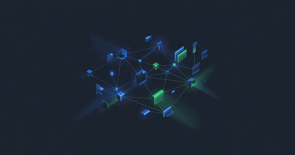
Semantic search solves this by embedding content into a high-dimensional vector space where meaning determines proximity, not word overlap. A query for “gradual shift in tone from supportive to controlling” will find relevant passages even if none of those exact words appear in the source material.

This isn’t theoretical. The pipeline is running in production against a real archive. It processes text messages, emails, voice recordings, and video transcripts spanning over a decade. The first complete run produced findings that eight independent analytical frameworks all converged on — patterns that would have taken months to surface manually.

Here’s how it works.

The Three-Machine Topology

The archive is too large and the compute requirements too varied for a single machine. The system spans three dedicated machines, each optimized for its role:

┌─────────────────────────┐       ┌─────────────────────────┐
│    Archive Server       │       │    GPU Workstation      │
│    28TB cold storage    │       │    RTX 3080 Ti (12GB)   │
│                         │       │                         │
│  iPad/iPhone backups    │       │  Whisper transcription  │
│  Camera footage         │       │  LLM orchestration      │
│  Voice recordings       │       │  Qdrant vector DB       │
│  YouTube archive        │       │  Pipeline scripts       │
│  Email/SMS exports      │       │                         │
└───────────┬─────────────┘       └────────────┬────────────┘
            │                                  │
            │     Direct Ethernet Link         │
            │◄────────────────────────────────►│
            │                                  │
            │         ┌────────────────────┐   │
            │         │  Editing Machine   │   │
            │         │  Apple Silicon     │   │
            │         │                    │   │
            │         │  NLE Software      │   │
            │         │  FCPXML bridge     │   │
            │         │  Local inference   │   │
            └────────►│                    │◄──┘
                      └────────────────────┘

Archive server: Holds everything. iPad backup folders dating back years. Camera footage from DSLRs and drones. Hundreds of voice recordings. A 129GB YouTube archive. Email exports. Text message databases. This machine’s job is to never lose anything. It stores raw media that has never been organized — the pile IS the input.

GPU workstation: The compute engine. An RTX 3080 Ti handles Whisper transcription (voice-to-text at 23-33x realtime using large-v3-turbo, which fits in ~6GB VRAM). It runs the embedding models through a local Ollama instance. It hosts the Qdrant vector database. And it orchestrates the LLM calls for summarization and synthesis. Every stage of the pipeline runs here.

Editing machine: Apple Silicon for native NLE performance. This is where the output of the pipeline becomes usable film — FCPXML files that describe timelines the editor can open, review, and modify. The editing machine talks to the GPU workstation to run queries and get back assembled clip lists.

The machines connect over direct ethernet. The archive server is essentially a giant NAS that the GPU workstation pulls raw media from as needed. Once media is transcribed and embedded, the archive server’s job is done — all subsequent queries hit the vector database on the GPU workstation.

This topology matters because it means each machine can be sized for its actual job. The archive server needs storage capacity, not GPU power. The GPU workstation needs VRAM, not 28TB of disk. The editing machine needs a display engine and NLE performance, not a vector database.

Stage 1: Ingestion — Collect the Pile

The first decision is the most important one: don’t organize anything. Just collect.

sources/
├── sms/           # Text message exports
├── email/         # Gmail API pulls, MBOX from Google Takeout
├── voice/         # M4A/MP4 from iPhone/iPad via cloud sync
├── therapy/       # Session recordings
├── docs/          # Legal documents, court filings, witness statements
└── video/         # Camera footage, drone passes, screen recordings

A sources.json config declares where each source type lives and maps files to contacts (the people involved in each conversation):

{
  "contacts": {
    "person-a": {
      "name": "Person A",
      "sources": [
        { "type": "sms", "path": "~/sources/sms/person-a.txt", "primary": true },
        { "type": "voice", "path": "~/sources/voice/person-a/", "primary": true },
        { "type": "email", "path": "~/sources/email/person-a.mbox", "primary": true }
      ]
    }
  }
}

The primary flag prevents double-counting when the same conversation appears in multiple export formats. Only primary sources get chunked.

Voice recordings need transcription before they can enter the text pipeline. Whisper large-v3-turbo running on the GPU workstation handles this at roughly 30x realtime — a 10-minute voice memo transcribes in about 20 seconds. The turbo variant is critical: the full large-v3 model exceeds 12GB VRAM and out-of-memory kills on the 3080 Ti. The turbo model fits comfortably in ~6GB with negligible quality loss.

The key principle at this stage: dump everything, curate nothing. The pipeline’s job is to find the signal in the noise. Human curation at the ingest stage means human bias at the ingest stage.

Stage 2: Chunking — Breaking Media into Searchable Units

Raw media files are too large to embed meaningfully. A 6-month text message history is tens of thousands of messages. A voice recording is 45 minutes of continuous speech. Embedding these as monolithic documents produces vectors that represent the average of everything, which means they match nothing well.

The chunking strategy: one chunk = one contact + one time period + one media type.

// Simplified chunking logic
function chunkByContactAndMonth(messages, contactId) {
  const months = groupByMonth(messages);
  
  return Object.entries(months)
    .filter(([_, msgs]) => msgs.length >= MIN_MESSAGES_PER_MONTH)
    .map(([period, msgs]) => ({
      contact: contactId,
      period,        // e.g., "2024-06"
      type: 'sms',
      tier: 'raw',
      content: msgs.map(m => `[${m.date}] ${m.sender}: ${m.text}`).join('\n'),
    }));
}

Each chunk gets structured frontmatter:

---
contact: person-a
period: 2024-06
type: sms
tier: raw
source: sources/sms/person-a.txt
date_range: 2024-06-01 to 2024-06-30
message_count: 47
---

[2024-06-01 09:12] Person A: ...
[2024-06-01 09:15] Me: ...
...

The tier field is important — it tracks where this document sits in the abstraction hierarchy. Raw chunks are tier raw. We’ll build three more tiers on top of them.

A few design decisions worth noting:

Minimum message threshold. Months with fewer than 3 messages get merged into adjacent months. A single text in July doesn’t warrant its own chunk — it’s noise that would dilute the embedding.

Contact normalization. Whisper mangles names. Text exports use phone numbers. Email uses addresses. The config maps all of these to a canonical contact ID so that “Mom,” “+1-555-0123,” and “s.johnson@email.com” all resolve to the same person.

Voice chunk boundaries. Voice recordings are chunked by individual file, not by time window. A 45-minute recording stays as one chunk because the semantic coherence of a single conversation matters more than artificial time boundaries. These chunks are the largest, often exceeding the embedding model’s context window — the embedder truncates to 6,000 characters (conservative for 8,192-token context) and the full text is stored in the payload for retrieval.

First run stats: 225 chunks across 8 contacts, spanning a decade of communications.

Stage 3: Summarization — AI First Pass

Each chunk gets a Grok-generated summary. This isn’t a simple text condensation — it’s a structured extraction of themes, dynamics, and notable quotes.

The summarization prompt asks the model to extract:

Key themes and topics discussed
Notable direct quotes (exact words matter for evidence)
Emotional tone and register shifts
Relationship dynamics (who has power, who accommodates, who deflects)
Anything significant from a narrative or analytical perspective

// pass2-summarize.mjs — simplified
async function summarizeChunk(chunk) {
  const prompt = `Summarize this ${chunk.type} exchange between ${chunk.contact} ` +
    `and the subject during ${chunk.period}. ` +
    `Extract key quotes, themes, emotional dynamics, and anything ` +
    `significant in a documentary or analytical context.`;
  
  const summary = await grokAPI(prompt, chunk.content);
  
  return {
    ...chunk,
    tier: 'summary',
    content: summary,
  };
}

Model selection matters here. This stage uses a fast, non-reasoning model because it’s volume work — 225 chunks need summarization, and the quality bar is “accurate extraction,” not “deep analysis.” Reasoning models are saved for later stages where cross-referencing and synthesis require genuine inference. Total API cost for summarization: about $2-3.

The output summaries become their own documents with tier: summary, stored alongside the raw chunks. Both tiers get embedded later — raw chunks are best for finding specific evidence, summaries are best for thematic queries.

Stage 4: Panorama — Cross-Contact Synthesis

This is where the archaeology begins.

Individual chunks and summaries show you one conversation at a time. Panoramas show you everything that was happening simultaneously across all relationships for a given time period.

Month: June 2024
├── Person A: [summary of their messages]
├── Person B: [summary of their messages]
├── Person C: [summary of their voice recordings]
└── Person D: [summary of their emails]
                    │
                    ▼
         PANORAMA: Cross-contact synthesis
         "During June 2024, three separate relationships
          exhibited the same behavioral pattern..."

The synthesis prompt feeds all contact summaries for a given month into a reasoning model and asks: What patterns emerge across relationships? What was happening from multiple directions simultaneously?

This stage uses a reasoning model because it needs to cross-reference and identify patterns that no individual summary contains. The model must hold five or six summaries in context and find the signal that cuts across them.

This is where the system earns its keep. Individual conversations look isolated. A text exchange feels like a one-off argument. An email feels like a specific grievance. But when you see three different people, in three different communication channels, exhibiting the same behavioral pattern during the same month — that’s not coincidence. That’s structure. And no human can hold 225 chunks in their head to see it.

First run stats: 187 panoramic syntheses.

Stage 5: Arcs — Character Trajectories and Pattern Atlas

The arc stage operates at the highest level of abstraction. It reads all panoramas and summaries for each contact and distills the full relationship trajectory — from beginning to present.

Output types:

Contact arcs (one per person): The complete arc of a relationship — how it started, how it evolved, what patterns emerged, where it stands now
Pattern atlas (one): Cross-cutting behavioral patterns that appear across multiple contacts, regardless of the specific relationship
Master timeline (one): A chronological spine of significant events, dates, and turning points

These arcs become tier: arc documents. They’re the most abstract tier and the least useful for finding specific evidence, but they’re invaluable for contextual queries — “what was the overall trajectory of this relationship?” maps naturally to arc-tier documents.

Stage 6: Embedding — Into the Vector Space

Every document from every tier gets embedded into a Qdrant vector database. The embedding model is nomic-embed-text, a 768-dimensional model running locally through Ollama.

// lib/embedder.mjs — core embedding logic
const EMBED_MODEL = 'nomic-embed-text';
const VECTOR_SIZE = 768;
const MAX_EMBED_CHARS = 6000;

export async function embed(text) {
  const truncated = text.length > MAX_EMBED_CHARS 
    ? text.slice(0, MAX_EMBED_CHARS) 
    : text;
    
  const res = await fetch('http://localhost:11434/api/embed', {
    method: 'POST',
    headers: { 'Content-Type': 'application/json' },
    body: JSON.stringify({ model: EMBED_MODEL, input: truncated }),
  });
  
  const data = await res.json();
  return data.embeddings[0];
}

export async function upsertDocument(id, text, metadata) {
  const vector = await embed(text);
  
  await qdrant.upsert(COLLECTION, {
    wait: true,
    points: [{
      id,
      vector,
      payload: { text: text.slice(0, 5000), ...metadata },
    }],
  });
}

Each document’s payload carries structured metadata: tier, contact, period, type, source_file, and an ISO timestamp extracted from the period string. This metadata enables filtered searches — “show me only raw SMS from Person A during 2024” is a metadata filter, not a semantic query.

The embedding runs locally. No API calls, no data leaving the machine. For a personal archive containing private communications, this is non-negotiable. The embedding model sits in Ollama’s cache, loaded once and held in memory. 645 documents embed in a few minutes.

The collection structure:

Collection: communications
├── Vectors: 768-dimensional, cosine distance
├── Documents: 645
├── Tiers:
│   ├── raw: ~225 (original chunks)
│   ├── summary: ~225 (AI summaries)
│   ├── panorama: ~187 (cross-contact syntheses)
│   └── arc: ~10 (relationship arcs + pattern atlas)
└── Payload: text (truncated), contact, period, type, tier, timestamp

The critical design choice: embed all tiers. Don’t just embed raw text and call it done. Each tier captures a different level of abstraction, and different queries benefit from different tiers. A query for a specific quote (“the exact words they used when…”) finds its best match in raw chunks. A query for a behavioral pattern (“gradual escalation of control”) matches best against panoramas or arcs. By embedding everything, the system automatically returns the right level of abstraction for each query.

Choosing an Embedding Model

Not all embedding models are created equal, and the choice matters more than most people realize. I benchmarked three models against a ground-truth test set with known correct answers:

Model	R@1	MRR	Dimensions	Query Latency	Notes
bge-m3	1.000	1.000	1024	808ms	Perfect retrieval, 27x slower
mxbai-embed-large	0.917	0.958	1024	28ms	Near-perfect, fast
nomic-embed-text	0.833	0.903	768	30ms	Good, fastest

R@1 is Recall at 1 — did the correct document rank first? MRR is Mean Reciprocal Rank — how high did it rank on average?

The telling misses were instructive. Both nomic and mxbai confused semantically similar but distinct entities in specialized domains. When the test query described “a spirit that understands the songs of birds and the speech of animals,” the general-purpose models mapped it to the wrong entity — they matched on surface-level vocabulary (“spirit,” “commands”) rather than the specific semantic content. bge-m3, trained on harder negative pairs and cross-lingual data, resolved every distinction correctly.

The tradeoff is real. bge-m3 is 27x slower per query. For an index-once, query-many workflow like this pipeline, that’s acceptable — you embed 645 documents once, then query interactively. But for high-volume real-time search (thousands of queries per second), nomic or mxbai at 28-30ms is the right choice.

My recommendation:

Specialized corpora (legal filings, archival material, mixed-language transcripts, domain-specific terminology): Use bge-m3. The retrieval quality gap on fine semantic distinctions is worth the latency.
General English at scale (chat RAG, product search, documentation): Use mxbai-embed-large. It’s nearly as good as bge-m3 and 27x faster.
Budget or legacy systems (768-dim collections already in production): nomic-embed-text is solid and has the smallest vector footprint.

Migration warning: Switching from a 768-dimensional model to a 1024-dimensional model requires recreating the collection and re-embedding every document. It’s not a parameter change — it’s a rebuild. Plan accordingly.

The Query Layer: Six Tools for Different Questions

Once the archive is embedded, querying it becomes the primary interface. I built six specialized query tools, each designed for a different type of question:

Semantic Search (`query.mjs`)

The basic tool. Type a natural language question, get the most semantically similar documents.

node scripts/query.mjs "language shifting from supportive to accusatory"

━━━ Result 1 ━━━  score: 0.7234  |  person-a  |  summary  |  sms  |  2025-02
  Source: data/summaries/person-a/2025-02.summary.md

  During February 2025, Person A's messaging pattern shifted markedly.
  Earlier exchanges maintained a supportive tone ("I'm always here for
  you," "you know I've got your back"), but by mid-month the language
  began incorporating diagnostic framing...
  [...truncated, use --full to see all]

Filters narrow the search space:

node scripts/query.mjs "financial pressure" --contact person-b --tier raw --type email

Evidence Assembly (`evidence.mjs`)

When you have a specific claim and need to find corroborating evidence. Uses multi-tier retrieval with weighted scoring:

// Tier weights — raw evidence is most valuable for corroboration
const TIER_WEIGHTS = {
  raw: 1.2,      // Primary source — strongest evidence
  summary: 1.0,  // AI analysis of primary source
  panorama: 0.8, // Cross-contact synthesis
  arc: 0.7,      // High-level narrative
};

// Multiple independent sources = stronger evidence
const CONTACT_DIVERSITY_BONUS = 0.1;

The evidence score combines semantic similarity with tier weight and a diversity bonus for multi-source corroboration. A claim supported by raw SMS from one person AND raw voice recordings from another person scores higher than the same claim supported by two summaries from the same person.

node scripts/evidence.mjs "systematic pattern of financial restriction"

  EVIDENCE ASSEMBLY
  Claim: "systematic pattern of financial restriction"
  Searching 30 candidates across all tiers...

  Found: 30 candidates → 10 strongest
  Sources: person-a, person-b, person-c
  Tiers: raw, summary, panorama
  Types: sms, voice, email
  Contact diversity: 3 independent sources

  Evidence strength: STRONG
  ████████████████████████████████░░░░░░░░ 0.7891

  ━━━ Evidence 1 ━━━  strength: 0.8234  |  person-a  |  raw  |  sms  |  2024-08
  ...

  ━━━━━━━━━━━━━━━━━━━━━━━━━━━━━━━━━━━━━━━━━━━━━━━━━━━━━━━━━━━━
  CORROBORATION CHAIN
  ━━━━━━━━━━━━━━━━━━━━━━━━━━━━━━━━━━━━━━━━━━━━━━━━━━━━━━━━━━━━

  person-a: 5 corroborating docs (best: 0.8234)
  person-b: 3 corroborating docs (best: 0.7456)
  person-c: 2 corroborating docs (best: 0.6891)

  3 independent sources corroborate this claim.

Cross-Contact Comparison (`compare.mjs`)

Same concept, different voices. How do different people in the archive describe the same phenomenon?

node scripts/compare.mjs "boundary setting" --contacts person-a,person-b,person-c

This reveals whether a pattern is isolated to one relationship or systemic across several. When three people independently describe the same dynamic using different words, the convergence is striking.

Temporal Evolution (`timeline.mjs`)

How did a theme evolve over time within a specific relationship?

node scripts/timeline.mjs "expressions of support" --contact person-a

Returns results sorted chronologically rather than by relevance score. You can see language shifting month by month — the slow erosion of genuine warmth into performative reassurance, or the sudden absence of a theme that was previously constant.

Behavioral Drift (`drift.mjs`)

This is the most mathematically interesting tool. It computes the centroid (average vector) for two time windows and measures the cosine distance between them. The result is a single number quantifying how much a relationship changed.

function computeCentroid(vectors) {
  const dim = vectors[0].length;
  const sum = new Array(dim).fill(0);
  for (const vec of vectors) {
    for (let i = 0; i < dim; i++) sum[i] += vec[i];
  }
  return sum.map(x => x / vectors.length);
}

// Drift = 1 - cosine_similarity(before_centroid, after_centroid)
const drift = 1 - cosineSimilarity(beforeCentroid, afterCentroid);

node scripts/drift.mjs --contact person-a --before 2024-06 --after 2025-06

  CENTROID DRIFT ANALYSIS
  Contact: person-a
  Before: < 2024-06
  After:  >= 2025-06

  Before window: 18 documents
  After window:  14 documents

  ┌────────────────────────────────────────────────┐
  │  DRIFT: 0.2847                                 │
  │  ████████████████████████░░░░░░░░░░░░░░░░░░░░  │
  │  Similarity: 0.7153                            │
  │  SIGNIFICANT — relationship transformation     │
  └────────────────────────────────────────────────┘

  Window coherence:
    Before: 0.7234 (tight cluster)
    After:  0.5891 (moderate spread)

  ⚠ After window is less coherent — behavior became more erratic/varied

The coherence metric adds nuance. A tight “before” cluster that loosens “after” suggests someone whose behavior became less predictable. A loose “before” that tightens “after” suggests someone whose behavior became more rigid or repetitive. Both are meaningful signals.

Interpretation guide:

Drift < 0.10: Minimal change — stable relationship
Drift 0.10-0.20: Moderate shift — evolving dynamics
Drift 0.20-0.30: Significant change — relationship transformation
Drift > 0.30: Major drift — fundamentally different relationship

Evidence Brief Compiler (`build-brief.mjs`)

The automated version of “compile the strongest evidence for a specific set of claims.” Takes a JSON config defining patterns to search for, runs dozens of targeted queries, deduplicates the results (cosine threshold > 0.85 to catch near-identical passages from different tiers), and assembles a structured brief under a configurable word budget.

node scripts/build-brief.mjs --config config/brief-subject.json --word-limit 3500

The config specifies query suites per pattern, contact filters, and retrieval limits. The compiler runs them all, tracks provenance, and produces a markdown document ready for the analysis battery.

The Analysis Battery: Multi-Framework Professional Assessment

The evidence brief feeds into an analysis battery — multiple independent professional frameworks, each analyzing the same evidence through a different lens.

Evidence Brief (3,500 words)
            │
     ┌──────┼──────┬──────┬──────┬──────┬──────┬──────┐
     ▼      ▼      ▼      ▼      ▼      ▼      ▼      ▼
  [Frame  [Frame [Frame [Frame [Frame [Frame [Frame [Frame
   work    work   work   work   work   work   work   work
    1]      2]     3]     4]     5]     6]     7]     8]
     │      │      │      │      │      │      │      │
     └──────┴──────┴──────┴──────┴──────┴──────┴──────┘
                           │
                           ▼
                   Convergence Matrix
                   Master Synthesis

Each framework gets its own API call with its own prompt. The evidence brief is identical across all calls — only the analytical lens changes. A clinical framework analyzes through diagnostic criteria. A legal framework evaluates evidence admissibility. A systems framework maps structural dynamics. No framework sees the output of any other framework.

This independence is critical. If you feed one framework’s output into the next, you get amplification, not validation. Independent convergence across different theoretical paradigms — when a clinical lens, a legal lens, and a systems lens all reach the same conclusion from the same evidence — is far more meaningful than any single framework’s assessment.

The anti-sycophancy problem is real. LLMs tend to confirm whatever the evidence brief implies. Every framework prompt includes adversarial instructions:

“Identify weaknesses and alternative explanations”
“First assume normal range. Only conclude deviation if evidence robustly overcomes this”
“Do not affirm any implied conclusion; reach your own based on your framework’s standards”

The first complete battery run: 8 independent frameworks, 8 convergent findings. ~$5-8 in API cost. The convergence matrix — showing which frameworks confirmed which patterns — is the single most powerful artifact the pipeline produces.

The “Aha” Moment: When the System Sees What You Can’t

Let me describe what it’s like to use this system.

You sit down with a question. Maybe it’s vague — “something changed around mid-2024.” You run a drift analysis. The number comes back: 0.28. Significant transformation. You didn’t imagine it.

So you dig. You run a timeline query against that contact, filtered to the six months before and after the drift point. The system returns passages you haven’t read in years — a text message from a Tuesday morning, a voice recording from a car ride, an email sent at 2 AM. Each one is individually unremarkable. A supportive phrase. An offer of help. A casual check-in.

But arranged chronologically by the timeline tool, a pattern emerges. The supportive phrases get shorter. The offers of help come with conditions. The check-ins start including subtle references to your mental state — not asking “how are you?” but telling you how you are.

You run a cross-contact comparison. “Boundary-setting responses.” The system pulls passages from three different relationships. Three different people, three different communication channels, three different time periods. The language is different. The pattern is identical.

This is the moment the system justifies its existence. Not when it finds the document you were looking for — any search engine can do that. But when it reveals the structure you couldn’t see because you were too close to it, because you were living inside it, because no human brain can hold 645 documents in working memory and compute the centroid drift.

The panorama stage is where this crystallizes. Individual conversations look like isolated events. But when the system synthesizes all contacts for a single month and reports that three separate relationships exhibited the same behavioral pattern during the same four-week window — that’s not a search result. That’s an archaeological finding.

I built this system to find specific moments in footage. What it actually does is find stories that were always there, hidden in the pile, waiting for something patient enough to read everything and see the whole picture at once.

Operational Concerns

Privacy and Data Sovereignty

This pipeline processes some of the most sensitive data imaginable — private communications, therapy recordings, legal documents. The architecture makes a specific choice: nothing leaves the local network.

Embedding runs locally through Ollama (nomic-embed-text, loaded from disk)
Qdrant runs as a local container with bind-mounted storage
Transcription runs locally through Whisper
The only external API calls are to the summarization LLM, and those use a paid API with no training-on-input guarantees

The vector database itself is replicated to a second machine on the local network for backup, but never to any cloud service. Snapshots are created via Qdrant’s snapshot API and synced to physically controlled storage.

For anyone building a similar system with sensitive data: treat the Qdrant storage directory like you’d treat the source files. It contains embedded representations of private content, and while you can’t reconstruct the original text from a 768-dimensional vector, the payloads store truncated text directly. Protect that directory.

Backup and Disaster Recovery

The raw data is king. Chunks, summaries, panoramas, and arcs live as markdown files in a data/ directory. If the Qdrant database is lost, a full re-embed from the data directory reconstructs it in minutes:

# Nuclear option: re-embed everything from source files
node scripts/embed.mjs

Qdrant snapshots provide faster recovery:

# Create snapshot
curl -X POST http://localhost:6333/collections/communications/snapshots

# Restore on a fresh instance
curl -X PUT 'http://localhost:6333/collections/communications/snapshots/recover' \
  -H 'Content-Type: application/json' \
  -d '{"location": "file:///qdrant/snapshots/snapshot.snapshot"}'

The data pipeline is deterministic — same inputs produce the same chunks. The summarization stage is not (LLM outputs vary), but summaries are stored as files, so they survive any database failure. The only truly irreplaceable assets are the original source files on the archive server.

Cost

The entire pipeline runs on hardware I already owned, with minimal API cost:

Stage	Model	Cost
Transcription	Whisper (local)	$0
Chunking	Custom scripts	$0
Summarization	Grok API (fast model)	~$2-3
Synthesis	Grok API (reasoning model)	~$3-5
Embedding	nomic-embed-text (local)	$0
Analysis Battery	Grok API (reasoning model)	~$5-8
Total		~$10-15

The first complete run — from raw, unorganized media pile to master evidence synthesis with 8 independent professional frameworks — cost about $12 in API calls. The infrastructure cost is in the machines, but those serve other purposes too. The GPU workstation runs AI inference for other projects. The archive server is a general-purpose NAS. Only the pipeline code and the Qdrant instance are dedicated to this system.

What I’d Do Differently

Start with bge-m3 for the embeddings. I used nomic-embed-text because it was fast and already running in Ollama. It’s good enough — 0.833 R@1 on my benchmark. But bge-m3’s perfect recall on specialized domains would have saved me from a few queries that returned close-but-wrong results. The 27x latency penalty doesn’t matter for an index-once workflow. I’ll migrate when I rebuild the collection, but it means re-embedding all 645 documents, which is why I haven’t done it yet.

Build the drift tool first. I built it last because it felt like a luxury. It turned out to be the single most useful tool in the suite. A single number — 0.28 — told me more than hours of manual review. If I were starting over, centroid drift would be the first query tool I build after basic semantic search.

Chunk voice recordings more aggressively. I kept each recording as a single chunk, which means 45-minute conversations get truncated at embed time. Breaking them into 5-minute sliding windows with 1-minute overlap would produce better vector representations at the cost of more documents. The current approach works because the payload stores the full text even when the embedding is based on the truncated version — but the search quality for long recordings is noticeably lower than for text messages, which are naturally small.

Automate the panorama-to-insight loop. The pipeline currently stops at “here are the documents.” The next frontier is closing the loop: query results feed into an LLM that generates follow-up queries based on what it found, iterating until it converges on a stable set of findings. This is essentially an autonomous research agent with the Qdrant database as its knowledge base. The infrastructure supports it — the tooling just needs the orchestration layer.

The Complete Stack

Component	Technology	Purpose
Transcription	Whisper large-v3-turbo (local, ~6GB VRAM)	Voice and video to text
Chunking	Custom Node.js scripts	Structure raw media by contact, period, type
Summarization	Grok API (fast model)	First-pass thematic extraction
Cross-contact synthesis	Grok API (reasoning model)	Panoramic monthly views
Arc generation	Grok API (reasoning model)	Relationship trajectories
Embedding	nomic-embed-text via Ollama (768-dim)	Local vector generation
Vector database	Qdrant (containerized, local)	Cosine similarity search + metadata filtering
Query tools	Custom Node.js (6 specialized scripts)	Semantic search, evidence, comparison, drift
Analysis	Grok API (reasoning model)	Multi-framework professional assessment
Master synthesis	Custom Node.js + human review	Convergence matrix, final document

Pipeline flow:

Raw Media → Chunk → Summarize → Panorama → Arc → Embed
                                                    │
                                                    ▼
                                          Query → Evidence Brief
                                                    │
                                                    ▼
                                          Analysis Battery → Master Synthesis

Time from raw media pile to master synthesis: about 4 days. Most of that is human review, not compute. The pipeline stages themselves complete in hours.

Closing Thoughts

The thing about 28 terabytes of personal media is that it contains stories you’ve already forgotten. Not just the big events — those you remember. It’s the small shifts. The week a relationship changed. The conversation where someone said the quiet part out loud and you didn’t register it at the time because you were living through it.

Semantic search doesn’t just make that media accessible. It makes it legible in a way that wasn’t possible before. The vector space doesn’t care about chronology or context or emotional attachment. It cares about meaning. And when you ask it a question and it returns a passage from three years ago that perfectly answers a question you couldn’t have articulated three years ago — that’s when you understand what this technology is actually for.

It’s not about finding files faster. It’s about finding the story in the pile.